What is a Decision Tree Machine Learning Model? Complete Guide with Examples

🌳 What is a Decision Tree Machine Learning Model?

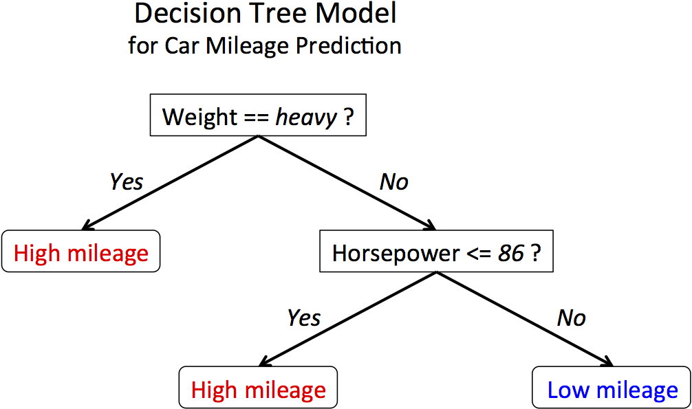
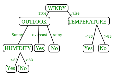
A Decision Tree is a powerful and intuitive supervised machine learning algorithm that mimics human decision-making processes. Imagine you're deciding whether to play tennis based on weather conditions - you might ask: "Is it sunny?" If yes, "Is the humidity high?" This chain of questions forms a tree-like structure, which is exactly how a Decision Tree works!

Key Characteristics: • Tree Structure: Resembles an upside-down tree with a root, branches, and leaves • Supervised Learning: Learns from labeled training data • Versatile: Used for both classification (predicting categories) and regression (predicting numbers) • Interpretable: Easy to understand and visualize • Non-parametric: Makes no assumptions about data distribution

🎯 Core Components of a Decision Tree: • Root Node: The starting point representing the entire dataset • Internal Nodes: Represent tests/questions on features (e.g., "Age > 25?") • Branches: Represent the outcome of tests (Yes/No paths) • Leaf Nodes: Final predictions or class labels • Depth: The length of the longest path from root to leaf • Pruning: Removing branches to prevent overfitting

📊 How is a Decision Tree Used in Classification?

Classification with Decision Trees is like playing "20 Questions" with your data. The algorithm systematically asks questions about features to separate different classes as cleanly as possible.

Classification Process:

1. Feature Selection: Choose the best feature to split on at each node
2. Threshold Determination: Find optimal cutoff values for continuous features
3. Data Partitioning: Split data into subsets based on feature values
4. Recursive Building: Repeat the process for each subset
5. Stopping Criteria: Stop when nodes are pure or meet other conditions
6. Prediction: Follow the path from root to leaf for new samples

🔍 Real-World Classification Example:

Email Spam Detection: • Root: "Does email contain word 'free'?" • Yes → "Are there more than 5 exclamation marks?" • Yes → SPAM (Leaf) • No → "Is sender in contact list?" • Yes → NOT SPAM (Leaf) • No → SPAM (Leaf) • No → "Does email have attachments?" • Yes → "Is attachment executable?" • Yes → SPAM (Leaf) • No → NOT SPAM (Leaf) • No → NOT SPAM (Leaf)

⚙️ How Does a Decision Tree Work? Step-by-Step Algorithm

The CART Algorithm (Classification and Regression Trees):

Step 1: Initialize • Start with entire training dataset at root node • Set current impurity measure (Gini or Entropy)

Step 2: Feature Selection Loop For each feature and possible split value: • Calculate impurity reduction (Information Gain) • Track the best split that maximizes information gain

Step 3: Split Decision • Choose feature and threshold with highest information gain • Create child nodes based on the split condition • Assign data samples to appropriate child nodes

Step 4: Recursive Construction • Repeat Steps 2-3 for each child node • Continue until stopping criteria are met:

• Maximum depth reached
• Minimum samples per node threshold
• All samples in node belong to same class
• No further improvement in impurity

Step 5: Pruning (Optional) • Remove branches that don't improve validation performance • Prevent overfitting to training data

🏗️ What is a Decision Tree? Detailed Structure

A Decision Tree is more than just a flowchart - it's a sophisticated data structure that encodes decision-making logic:

Tree Components Explained: • Nodes: Decision points that contain:

• Feature name to test
• Threshold value for split
• Impurity measure
• Number of samples
• Class distribution

• Edges/Branches: Represent outcomes of tests

• Binary splits: True/False, ≤/>threshold
• Multi-way splits: Categorical features

• Leaves: Terminal nodes containing:

• Final class prediction
• Confidence/probability scores
• Sample count for prediction

🎨 Advantages and Disadvantages

✅ Advantages: • Interpretability: Easy to understand and explain • No Data Preprocessing: Handles missing values and mixed data types • Feature Importance: Automatically identifies important features • Non-linear Relationships: Can capture complex patterns • Fast Prediction: Quick inference for new samples

❌ Disadvantages: • Overfitting: Prone to memorizing training data • Instability: Small data changes can create very different trees • Bias: Favors features with more split points • Limited Expressiveness: Struggles with linear relationships • High Variance: Performance varies significantly across datasets

🧮 What Math is Involved in Decision Trees? (Step-by-Step Guide)

Decision Trees use mathematics to make smart decisions about how to split data. Think of it like a smart calculator that finds the best questions to ask! Let's break it down into easy steps:

📚 The Math Building Blocks:

Step 1: Understanding Probability • If you have 10 apples and 6 are red, the probability of picking a red apple is 6/10 = 0.6 • This basic concept is used everywhere in decision trees!

Step 2: Measuring "Messiness" (Impurity) • Imagine a box with mixed colored balls - how mixed is it? • Pure box = all same color (easy to predict) • Mixed box = many colors (hard to predict)

Step 3: Finding the Best Split • Try different ways to separate the data • Pick the method that creates the "cleanest" groups • Use math to measure which split is best

🎲 Step 1: What is Gini Impurity? (Made Simple)

Gini Impurity is like measuring how "messy" a group is. Named after Italian statistician Corrado Gini, it tells us the chance of making a wrong guess.

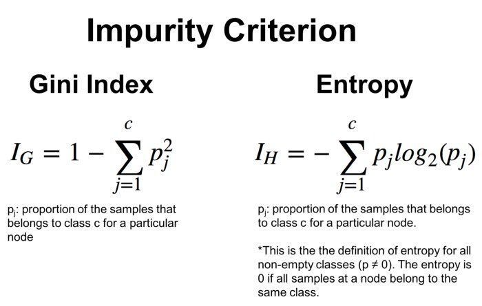
🔢 The Formula (Don't Worry, We'll Break It Down!):

$$Gini = 1 - \sum_{i=1}^{n} p_i^2$$

Let's Solve This Step by Step:

Example: A Classroom with Students Imagine a class of 100 students: • 60 like Math (Class A) • 40 like Science (Class B)

Step 1: Calculate Probabilities • P(Math) = 60/100 = 0.6 • P(Science) = 40/100 = 0.4

Step 2: Square Each Probability • P(Math)² = 0.6 × 0.6 = 0.36 • P(Science)² = 0.4 × 0.4 = 0.16

Step 3: Add Them Up • Sum = 0.36 + 0.16 = 0.52

Step 4: Apply Gini Formula • Gini = 1 - 0.52 = 0.48

🎯 What Does Gini = 0.48 Mean? • Gini = 0: Perfect! Everyone likes the same subject • Gini = 0.5: Maximum messiness (50-50 split) • Gini = 0.48: Pretty mixed, but not the worst

🔍 Step 2: Understanding Entropy (Information Theory Made Easy)

Entropy measures how much "surprise" or "uncertainty" is in your data. Think of it like this: if you can easily guess the answer, entropy is low. If it's hard to guess, entropy is high!

🔢 The Entropy Formula:

$$Entropy = -\sum_{i=1}^{n} p_i \times \log_2(p_i)$$

Let's Use the Same Classroom Example:

Step 1: Start with Probabilities (Same as Before) • P(Math) = 0.6 • P(Science) = 0.4

Step 2: Calculate Log Values • log₂(0.6) = -0.737 (don't worry about how, just use a calculator!) • log₂(0.4) = -1.322

Step 3: Multiply Probability × Log • Math part: 0.6 × (-0.737) = -0.442 • Science part: 0.4 × (-1.322) = -0.529

Step 4: Add Them and Make Positive • Sum = -0.442 + (-0.529) = -0.971 • Entropy = -(-0.971) = 0.971

🎯 What Does Entropy = 0.971 Mean? • Entropy = 0: No surprise! Everyone likes the same thing • Entropy = 1: Maximum surprise (50-50 split for 2 classes) • Entropy = 0.971: High uncertainty, close to maximum

⚖️ Step 3: Gini vs Entropy - Which is Better?

🏃‍♂️ Speed Race: • Gini Winner! Faster to calculate (no complex log functions) • Entropy: Slower but more mathematically precise

🎯 Sensitivity Test: • Entropy Winner! More sensitive to small changes • Gini: Less sensitive, more stable

📊 Practical Results: • Both usually create very similar decision trees • Most libraries use Gini as default (it's faster!) • Choose based on your needs: speed (Gini) vs precision (Entropy)

🔄 Quick Comparison Table:

| Measure | Our Example | Range | Best Value | Worst Value | |---------|------------|-------|------------|-----------| | Gini | 0.48 | 0 to 0.5 | 0 (pure) | 0.5 (mixed) | | Entropy | 0.971 | 0 to 1 | 0 (pure) | 1 (mixed) |

🎯 Step 4: Information Gain - Choosing the Best Split

Information Gain measures how much "cleaner" your groups become after a split. It's like asking: "Did this question help organize our messy data?"

🔢 The Information Gain Formula:

$$Information Gain = Original Impurity - Weighted Average of New Impurities$$

Or more precisely:

$$IG(Dataset, Feature) = Impurity(Dataset) - \sum \frac{|Subset|}{|Dataset|} \times Impurity(Subset)$$

📝 Real Example: Splitting Students by Age

Before Split (Original Dataset): • 100 students total • 60 like Math, 40 like Science • Gini = 0.48 (as calculated above)

After Split by Age > 18: • Group 1 (Age ≤ 18): 70 students

• 50 like Math, 20 like Science
• Gini₁ = 1 - [(50/70)² + (20/70)²] = 1 - [0.51 + 0.08] = 0.41

• Group 2 (Age > 18): 30 students

• 10 like Math, 20 like Science
• Gini₂ = 1 - [(10/30)² + (20/30)²] = 1 - [0.11 + 0.44] = 0.45

Calculate Information Gain: • Weighted Average = (70/100 × 0.41) + (30/100 × 0.45) = 0.287 + 0.135 = 0.422 • Information Gain = 0.48 - 0.422 = 0.058

🎯 What Does This Mean? • Positive gain (0.058) = Good split! Data became cleaner • Higher gain = Better split • Negative gain = Bad split, makes things messier

🔧 Step 5: What is Impurity? Connecting All the Math Together

Now that we understand Gini and Entropy, let's see how "Impurity" connects everything!

🎭 Impurity: The Master Concept Impurity is like measuring how "mixed up" or "messy" a group is:

📊 Visual Understanding: • Pure Node (Impurity = 0): 🟦🟦🟦🟦🟦 (All same class - Easy to predict!) • Mixed Node (High Impurity): 🟦🟨🟦🟨🟦 (Mixed classes - Hard to predict!) • Maximum Impurity: 🟦🟨🟦🟨🟨 (50-50 split - Hardest to predict!)

🔄 How Impurity Drives Decision Trees:

Step A: Start with Messy Data • Root node has mixed classes (high impurity) • Goal: Make it less messy!

Step B: Try Different Splits • Test various questions: "Age > 25?", "Income > $50k?" • Calculate impurity for each resulting group

Step C: Pick the Best Split • Choose the split with maximum Information Gain • Information Gain = How much cleaner the groups become

Step D: Repeat Until Clean • Keep splitting until groups are pure (or close enough) • Each split reduces overall impurity

🎯 Why This Math Matters:

1. Split Selection: Math finds the best questions to ask
2. Stopping Rules: Stop when impurity is low enough
3. Tree Quality: Lower impurity = Better predictions
4. Automated Process: Computer does all the math for us!

🔗 The Beautiful Connection: • Impurity measures messiness • Gini & Entropy are different ways to calculate impurity • Information Gain measures impurity reduction • Decision Tree automatically finds splits that maximize gain

It's like having a super-smart organizer that automatically finds the best way to sort your data! 🧠✨

🔗 Code Examples and Jupyter Notebook

For comprehensive hands-on experience with Decision Tree implementation, including: • Data preprocessing and exploration • Tree construction and visualization • Hyperparameter tuning • Performance evaluation • Comparison with other algorithms • Real-world datasets and case studies

Visit the complete GitHub repository:

🚀 Decision Tree Classifier - Complete Code & Notebook

The repository includes: • Jupyter notebooks with step-by-step explanations • Python scripts for different use cases • Dataset examples and preprocessing techniques • Advanced topics like ensemble methods • Performance comparison with other ML algorithms

🎯 Key Takeaways

• Decision Trees are intuitive, tree-like models perfect for classification and regression • Classification works by recursively splitting data based on feature values • Tree Construction uses mathematical measures like Gini impurity and entropy • Gini Impurity measures the probability of misclassification • Impurity represents how mixed classes are in a node • Mathematics involves information theory, probability, and optimization • Practical Implementation is straightforward with libraries like scikit-learn

Decision Trees remain one of the most important algorithms in machine learning due to their interpretability and effectiveness across various domains!

📚 Further Reading and Resources

• Books: "The Elements of Statistical Learning" by Hastie, Tibshirani & Friedman • Papers: Original CART algorithm by Breiman et al. (1984) • Online Courses: Machine Learning courses on Coursera, edX, and Udacity • Documentation: Scikit-learn Decision Tree documentation • Practice: Kaggle competitions and datasets

About the Author: This comprehensive guide was created by Zeeshan Ali, a passionate machine learning engineer. Connect with me on LinkedIn for more ML content and discussions!